Mapping public green spaces in Manchester

October 12, 2021

python geopandas matplotlib spatial-analysis open-data

The benefits of having public green areas around when living in a densely populated city are many, from encouraging exercise or providing spaces for socializing to decreasing noise and air pollution.

I aim to map public green areas in Manchester and how they distribute according to their population. Fields in Trust have done an amazing job at mapping the whole of the UK and establishing their green-space index, but I aim to have my own go at running a spatial analysis using python and geoPandas.

GIS and spatial analysis

GIS stands for Geographic Information System and it is a spatial system that enables the creation, management, analysis and mapping of all types of data. GIS allows to understand information within their geographic context, being able to spot geographical patterns, which would be very difficult to spot without the aid of a map. This type of analysis is called spatial analysis, and it is commonly used across many industries to discover patterns, incidents and coordinate spatial resources.

There are a few main concepts that is perhaps best to tackle first:

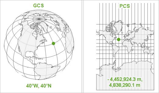
A geographic coordinate system (GCS) is a reference framework that defines the locations of features on a model of the earth. It’s shaped like a globe—spherical. Its units are angular, usually degrees.
A projected coordinate system (PCS) is flat. It contains a GCS, but it converts that GCS into a flat surface, by projecting points into the plane. Its units are linear, for example in meters. Note that not all projections conserve area, therefore two shapes with the same area on the globe may appear to be different in size after having been projected.

Where to find geo open data

For any piece of spatial analysis, the first thing you need is geographic data, ideally open source (unless your company is paying for it!). Geospatial data can come in many shapes (pun intended) and forms. Geospatial data files contain geometric location and any other associated attribute information. There are many different formats, but the most common ones are:

Esri Shapefile - the industry standard. A complete set of three files make up a shapefile: .shp is the feature geometry, .shx is the shape index positiona and .dbf is the attribute data.
Geographic JavaScript Object Notation (GeoJSON) - commonly used for web-based mapping. GeoJSON stores coordinates in JSON format. Extensions are .geojson and .json.

Other resources may just provide a raw flat csv file with a reference to a geographical area, like a postcode. A combination of that flat file and a geospatial file may be needed in these cases.

Government institutions usually collate and share geographical information at different granularities. In the UK, the Office for National Statistics and OrdenanceSurvey are your two main go-to places. In Manchester, Mapping GM is a great resource that collates geospatial data from different sources. But remember, Google is always your friend.

For this analysis, we have downloaded data from:

Geopandas for data manipulation

GeoPandas is a python library that enables geospatial data manipulation. It introduces the geoSeries, a subclass of pandas.Series, which handles the geometries (points, polygons etc.). The geoDataFrame extends the popular concept of a pandas.DataFrame by adding a geometry column, which specifies the geometry of each row in a geoSeries. The beauty of this class hierarchy is that you can store as much metadata in your geoDataFrame as you would in a regular DataFrame and you can keep using Pandas functionalities for data manipulation for free.

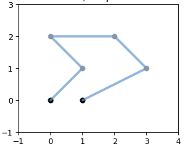
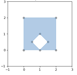
geoSeries make use of shapely geometry objects to specify their spatial boundaries.

There are three main types:

A point, coordinate values or point tuple parameters. Point(0.0, 0.0)
A line, an ordered sequence of 2 or more point tuples. LineString([(0, 0), (1, 1)])
A polygon, an ordered sequence of point tuples that form a closed polygon. It can also specify an optional unordered sequence of ring-like sequences specifying the interior boundaries or “holes” of the feature. Polygon([(0, 0), (1, 1), (1, 0)])

geoSeries also store information about the projection used to generate the coordinates (geoSeries.crs). A single geoDataFrame can contain multiple geoSeries with different CRS, which means you can store multiple projections of the same geospatial objects, although only one geometry will be considered as the active geometry for a specific geoDataFrame.

But, how does one use GeoPandas then? Well, I am glad you asked.

To start with, you need to read the geospatial file using geoPandas.read_file(), which automatically detects the file type and returns a geoDataFrame object.

import geopandas as gpd

fp = 'data/boundary_lines/district_borough_unitary_region.shp'
df = gpd.read_file(fp)

GeoPandas reading functionality is powered by the great fiona library, which in turn makes use of a massive open-source program called GDAL/OGR designed to facilitate spatial data transformations.

As our boundaries file contains boundary polygons for all districts in the UK, we need to filter down to only those of Greater Manchester. We can use regular Pandas functionality to do this:

greater_manchester_districts = [
    'Manchester District (B)',
    'Bury District (B)',
    'Oldham District (B)',
    'Rochdale District (B)',
    'Salford District (B)',
    'Trafford District (B)',
    'Stockport District (B)',
    'Tameside District (B)',
    'Bolton District (B)',
    'Wigan District (B)',
]

# Filtering to Greater Manchester
gmcr_boroughs = df[df['NAME'].isin(greater_manchester_districts)]

And lastly, for particular tasks, you may need to change the projection that your data comes in. For example, we need to use epsg=3857 (WGS 84 / Pseudo-Mercator) to be able to plot on top of contextly open maps. Luckily, changing the projection used is really easy with the geoDataFrame.to_crs() method.

gmcr_boroughs.to_crs(epsg=3857, inplace=True)

Green public areas in Greater Manchester

So far so good, but we need to upload geospatial data for green public areas within Greater Manchester. In our case, we know that Grater Manchester spreads across OrdnanceSurvey SD and SJ quadrants, so we need to read both files and concatenate the resulting geoDataFrames.

fp = 'data/greenspace_SD/SD_GreenspaceSite.shp'
gs_sd = gpd.read_file(fp)

fp = 'data/greenspace_SJ/SJ_GreenspaceSite.shp'
gs_sj = gpd.read_file(fp)

gs = gpd.GeoDataFrame(
    pd.concat([gs_sd, gs_sj], ignore_index=True)
)

We are only interested in certain types of green spaces, so we will filter down our geoDataFrame.

function_types = [
    'Play Space',
    'Playing Field',
    'Public Park Or Garden',
    'Bowling Green',
    'Allotments Or Community Growing Spaces',
]
gs = gs[gs['function'].isin(function_types)]

Still, gs will contain all polygons for quadrants SD and SJ. We can use geoPandas.overlay() function to intersect gs and gmcr_boroughs frames.

# Filtering down to green spaces in greater manchester
gmcr_gs = gpd.overlay(gmcr_boroughs, gs, how='intersection')

Mapping with matplotlib

Now we can finally plot these green spaces. GeoPandas can also plot maps with the aid of the geoDataFrame.plot() method which calls the matplotlib library.

gmcr_gs.plot()

The first time I manage to plot geospatial data, I was really excited. But quickly you realise that as maps go, this simple rendering of our geoDataFrame lacks the feel of a map. Let’s work on that.

Let’s start by defining the bounding box for the map. We can use shapely.ops.cascade_union function to union polygons that define Greater Manchester into one big polygon. Then we can use the geoSeries.bounds property to extract the minimum and maximum coordinates for the polygon.

from shapely.ops import cascaded_union

# Define Greater Manchester polygon
greater_manchester = gpd.GeoSeries(cascaded_union(gmcr_boroughs.geometry))

# Define bounding box
bounds = greater_manchester.bounds
bounding_box = [
    bounds['minx'][0],
    bounds['maxx'][0],
    bounds['miny'][0],
    bounds['maxy'][0],
]

# Set bounds
ax.set_xlim(bounding_box[0]-1000, bounding_box[1] + 1000)
ax.set_ylim(bounding_box[2]-1000, bounding_box[3] + 1000)

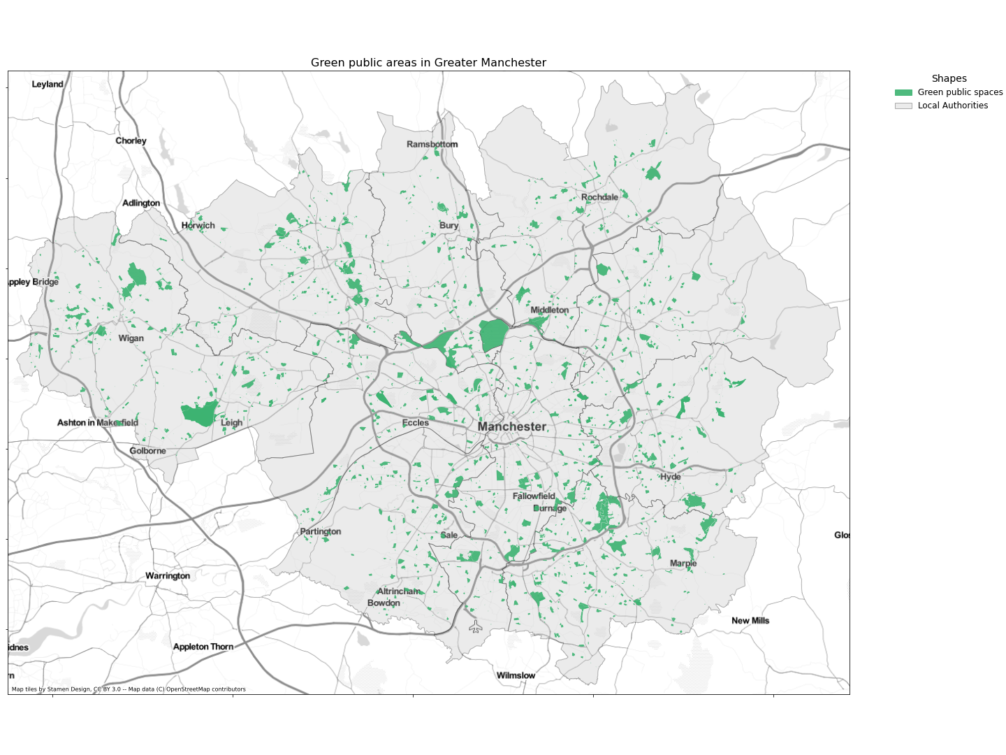
We then can go on and plot both the local authority boundaries (almost transparent, with alpha=0.3) and the green area polygons (as green shapes).

# Plot borough borders
gmcr_boroughs.plot(
    ax=ax, 
    alpha=0.3, 
    edgecolor='black', 
    facecolor='silver',
)

# Plot green areas
gmcr_gs.plot(
    ax=ax, 
    alpha = 0.9, 
    color='mediumseagreen',
    label='Green Open Spaces',
)

We can use contextily to add a background map, which enhances the geographic contextualisation.

import contextily as cx # map backgrounds

# Add background
cx.add_basemap(ax, source=cx.providers.Stamen.TonerLite)

Let’s also remove ticks from axes, as they no longer carry relevant meaning.

# Remove axis 
ax.set_yticklabels([])
ax.set_xticklabels([])

Last but not least, I want to add a legend. As the map layers we have added don’t provide legend handles, we will create them from scratch with the following few lines.

# Legend
import matplotlib.patches as mpatches
green_patch = mpatches.Patch(color='mediumseagreen', alpha=0.9, label='Green public spaces')
gray_patch = mpatches.Patch(facecolor='silver', edgecolor='black', alpha=0.3, label='Local Authorities')
leg = plt.legend(
    handles=[green_patch, gray_patch],
    bbox_to_anchor=(1.05, 1),
    loc=2,
    borderaxespad=0.,
    frameon=False,
    prop={'size': 12},

Putting it all together, we get this beauty of a map.

Running spatial calculations

Fantastic. But, what if we want to run more complex calculations. For example, what if we want to quantify the access to green public space based on population and break this down to a granular geographic breakdown, like postal sector? GeoPandas is here to help.

First, we need to read postal sector (the area corresponding to addresses that map to the same postal code without the last couple of letters, for example, all addresses starting with N3 5) shapes and reduce the frame to those of Greater Manchester. Let’s use geoPandas.readfile() and geoPandas.overlay() for this task.

# UK Postal Sector boundaries
fp = 'data/GB_Postcodes/PostalSector.shp'
ps = gpd.read_file(fp)
ps.to_crs(epsg=3857, inplace=True)

# Filter by postal sectors in greater manchester
gmcr_ps = gpd.overlay(gmcr_boroughs, ps, how='intersection')

We now need to quantify the area that each postal sector has access to. We want to calculate the amount of green spaces within a 10-minute walk from each postal district. Why 10 minutes? As the people from Fields in Trust brilliantly explain, a ten-minute walking distance is a well-established measure of an acceptable distance for a resident to be from their nearest park or green space. To make things easier, I will use the equivalent distance of a 10 minutes walk, which is roughly equivalent to 800 meters (Wikipedia: 10 min walk).

Firstly, let’s copy our GeoDataFrame, as we will need the actual postal sector boundaries as they are later on. Let’s use shapely.buffer() to expand out our geometry boundaries 800 meters.

gmcr_expanded_ps = gmcr_ps.copy()
gmcr_expanded_ps['geometry'] = gmcr_expanded_ps['geometry'].apply(lambda geo: geo.buffer(800))

shapely calculates the distance in a Euclidean manner, using the good old Pythagoras’s theorem. This is not a big problem if our analysis uses a projection that preserves areas, unlike Mercator. I will use the Equal-Area Scalable Earth Grid (EASE-Grid), epsg=6933.

gmcr_expanded_ps.to_crs(epsg=6933, inplace=True)
mcr_gs_ease = gmcr_gs.copy()
mcr_gs_ease.to_crs(epsg=6933, inplace=True)

Let’s loop over each expanded postal sector and calculate the intersection of our expanded boundary with all green areas within Greater Manchester. We can use shapely.intersection method to obtain the intersection between two polygons. We can then access the area of the resulting polygon by accessing the public area property.

gmcr_expanded_ps['green_area_sq_km'] = 0.0

for i, postal_sectors in gmcr_expanded_ps.iterrows():
    for j, green_space in enumerate(mcr_gs_ease['geometry']):
        green_area_in_postal_sector = postal_sectors['geometry'].intersection(green_space)
        gmcr_expanded_ps.at[i, 'green_area_sq_km'] += green_area_in_postal_sector.area / 10**6 # squared km

gmcr_expanded_ps['green_area_ha'] = gmcr_expanded_ps['green_area_sq_km'] * 100
gmcr_expanded_ps['green_area_sq_m'] = gmcr_expanded_ps['green_area_sq_km'] * 1000000

Excellent, let’s merge these are calculations back to our original geoDataFrame.

gmcr_ps = pd.merge(
    gmcr_ps,
    gmcr_expanded_ps,
    how='left',
    on='RMSect',
)

Now let’s add population data. Population data at postal sector level can be extracted from Nomis. I have extracted postal sector population (usual residents) for the whole of the North West, so I will have to filter the file down. This data is based on the 2011 Census, which is now 10 years old. Not ideal, but it is the only source of open population data at such a granular level. This data is contained in a CSV file, which has no geospatial reference other than the postal sector as a string. We need to transform this data a little bit.

pop = pd.read_csv(
    'data/2974730013.csv', 
    skiprows=11, 
    names=['area','population'],
)
# removing spaces from postal sector for an easier match
pop['StrSect'] = pop['area'].str[7:].str.replace(' ','')
pop.drop('area', axis=1, inplace=True)

# converting population to numeric
pop = pop[:-4]
pop['population'] = pop['population'].apply(pd.to_numeric)

Left join to our gmcr_ps geoDataFrame and calculate the area/inhabitants ratio.

gmcr_ps = pd.merge(
    gmcr_ps,
    pop,
    how='left',
    on='StrSect',
)

# calculate area/inhabitants ratio
gmcr_ps['green_area_sq_m_pp'] = gmcr_ps['green_area_sq_m']/gmcr_ps['population']

And now let’s plot these values. We can easily do that by indicating which column we want to use from the dataFrame.

# Plot green areas access
vmin, vmax = 0, 1200
gmcr_ps.plot(
    ax=ax, 
    column='green_area_sq_m_pp', 
    cmap='hot_r', 
    vmin=vmin, 
    vmax=vmax, 
    alpha=0.7,
)

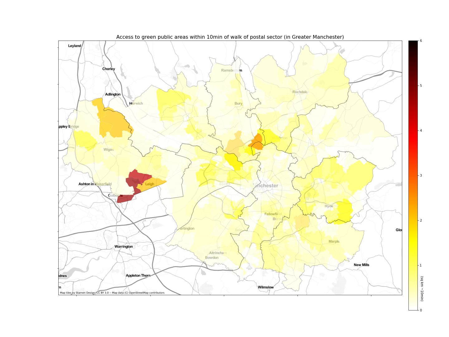
Beautiful! This type of chart is called a choropleth, a type of map in which regions is coloured or patterned in proportion to a variable that represents an aggregate summary of a geographic characteristic within the area.

To wrap-up

We have seen how python and geoPandas provide a great set of tools to perform GIS spatial analysis. Even underestimating its population because of using old census data, the centre of Greater Manchester comes up as severely underprovided for in terms of green public spaces.